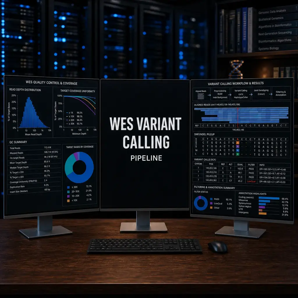
Whole Exome Sequencing (WES): Variant Calling & VAF

Whole Exome Sequencing (WES) Pipeline

Introduction

While RNA sequencing (RNA-seq) tells us what genes are actively expressed, Whole Exome Sequencing (WES) reveals the underlying DNA mutations. WES specifically targets the protein-coding regions of the genome, making it a highly cost-effective method for identifying disease-causing variants in cancer and rare genetic disorders.

This tutorial covers the standard bioinformatics pipeline for processing raw WES data, calculating Variant Allele Frequency (VAF), and managing genome assembly liftovers.

1. Raw Data Processing & Alignment

The first step in any DNA-seq pipeline is aligning the raw FASTQ reads to a reference genome (e.g., GRCh38/hg38) and marking PCR duplicates.

BWA-MEM Alignment

BWA-MEM is a widely used aligner for short DNA reads; follow your laboratory or project standard if another validated workflow is required.

# Index the reference genome (only needed once)
bwa index Homo_sapiens_assembly38.fasta

# Align paired-end reads to the reference
bwa mem -t 8 Homo_sapiens_assembly38.fasta sample_R1.fastq.gz sample_R2.fastq.gz > aligned_reads.sam

Sorting and Marking Duplicates (GATK / Picard)

We use samtools to convert to BAM, and Picard to remove PCR duplicates that arise during exome capture library preparation.

# Convert SAM to BAM and sort by coordinate
samtools sort -@ 8 -o sorted_reads.bam aligned_reads.sam

# Mark Duplicates
java -jar picard.jar MarkDuplicates \
      I=sorted_reads.bam \
      O=dedup_reads.bam \
      M=marked_dup_metrics.txt

2. Validate GATK Inputs and Recalibrate When Appropriate

Before calling variants, confirm that the reference build, aligned reads, known-sites resources, and metadata all refer to the same genome assembly. GATK requires key read-group fields, and missing metadata can cause failures or make technical interpretation unreliable.

# Reference prerequisites for GATK
samtools faidx Homo_sapiens_assembly38.fasta
gatk CreateSequenceDictionary -R Homo_sapiens_assembly38.fasta

# Inspect existing read groups. You should see @RG lines with ID, SM, LB, and PL fields.
samtools view -H dedup_reads.bam | grep '^@RG'

# Only if read groups are absent or incorrect, add values supplied by your sequencing facility.
gatk AddOrReplaceReadGroups \
  -I dedup_reads.bam -O dedup_reads.rg.bam \
  -RGID flowcell.lane -RGLB library1 -RGPL ILLUMINA -RGPU flowcell.lane.barcode -RGSM sample1

For human germline-style workflows with a compatible, trusted known-sites resource, use Base Quality Score Recalibration (BQSR) according to the current GATK Best Practices. Do not apply BQSR blindly when the required reference and known-sites assumptions are not met.

# Example only: use a known-sites VCF that matches exactly the same reference build.
gatk BaseRecalibrator \
  -R Homo_sapiens_assembly38.fasta \
  -I dedup_reads.rg.bam \
  --known-sites known_sites.vcf.gz \
  -O recalibration.table

gatk ApplyBQSR \
  -R Homo_sapiens_assembly38.fasta \
  -I dedup_reads.rg.bam \
  --bqsr-recal-file recalibration.table \
  -O recal_reads.bam

A successful preparation has a .fai file, a .dict file, readable @RG header lines, and a recalibration table when BQSR is used.

3. Variant Calling (GATK HaplotypeCaller)

Once inputs are aligned, deduplicated, and validated, use the Broad Institute's GATK (Genome Analysis Toolkit) to identify SNPs and indels.

# Use the BQSR output when BQSR was appropriate for the selected workflow.
gatk HaplotypeCaller \
     -R Homo_sapiens_assembly38.fasta \
     -I recal_reads.bam \
     -O raw_variants.vcf.gz

4. Variant Allele Frequency (VAF) Analysis

Variant Allele Frequency (VAF) is the percentage of sequencing reads matching a specific DNA variant divided by the total coverage at that locus. In cancer genomics, VAF is critical for determining whether a mutation is clonal (present in all tumor cells) or subclonal.

Calculating VAF in R

If you extract the allelic depths (AD) and total depth (DP) from your VCF into a data frame, you can analyze VAF in R:

library(ggplot2)
library(dplyr)

# Example: Read extracted VCF data
variant_data <- read.csv("extracted_variants.csv")

# Calculate VAF: Alternate Allele Depth (AD_alt) / Total Depth (DP)
variant_data <- variant_data %>%
  mutate(VAF = AD_alt / DP)

# Visualize the VAF distribution to look for clonal peaks
ggplot(variant_data, aes(x = VAF)) +
  geom_histogram(binwidth = 0.02, fill = "darkred", color = "black", alpha = 0.7) +
  theme_minimal() +
  labs(title = "Variant Allele Frequency (VAF) Distribution",
       x = "VAF",
       y = "Number of Mutations")

A peak near VAF = 0.5 can be consistent with heterozygous variants in an adequately covered diploid sample, but purity, copy-number change, allele-specific bias, and coverage alter observed VAF. Do not infer clonality or germline status from VAF alone.

5. Genome LiftOver (e.g., hg19 to hg38)

Often, you may receive older variant data mapped to an outdated genome assembly (like hg19). You must "LiftOver" these coordinates to the modern hg38 assembly before combining them with new data.

library(rtracklayer)
library(GenomicRanges)

# Load the chain file downloaded from UCSC
chain <- import.chain("hg19ToHg38.over.chain")

# Create a GRanges object of your hg19 variants
hg19_variants <- GRanges(seqnames = Rle(c("chr1", "chr2")),
                         ranges = IRanges(start = c(10000, 20000), width = 1))

# Perform the LiftOver
hg38_variants <- liftOver(hg19_variants, chain)

print(hg38_variants)

Conclusion

A robust WES pipeline requires careful alignment, stringent duplicate removal, accurate variant calling, and deep interpretation of metrics like VAF. By mastering these steps, you can confidently identify pathogenic mutations in complex cohorts.

Matched Python and R VAF calculation

Check the VCF header and sample order before calculating variant allele fraction. The simplified examples below use allele-depth fields and should be extended for multi-allelic sites, quality filters, tumor purity, and copy-number context.

import pandas as pd
from cyvcf2 import VCF

rows = []
for variant in VCF("sample.vcf.gz"):
    allele_depths = variant.format("AD")[0]
    if allele_depths is None or len(allele_depths) < 2:
        continue
    ref_depth, alt_depth = map(int, allele_depths[:2])
    total_depth = ref_depth + alt_depth
    rows.append({
        "chrom": variant.CHROM,
        "position": variant.POS,
        "vaf": alt_depth / total_depth if total_depth else float("nan"),
    })
vaf_table = pd.DataFrame(rows)

library(VariantAnnotation)

vcf <- readVcf("sample.vcf.gz")
allele_depths <- geno(vcf)$AD
ref_depth <- allele_depths[1, 1, ]
alt_depth <- allele_depths[2, 1, ]
vaf <- alt_depth / (ref_depth + alt_depth)
vaf_table <- data.frame(position = start(rowRanges(vcf)), vaf = vaf)