Downstream Analysis

Beyond Clustering: Functional Single-Cell Biology

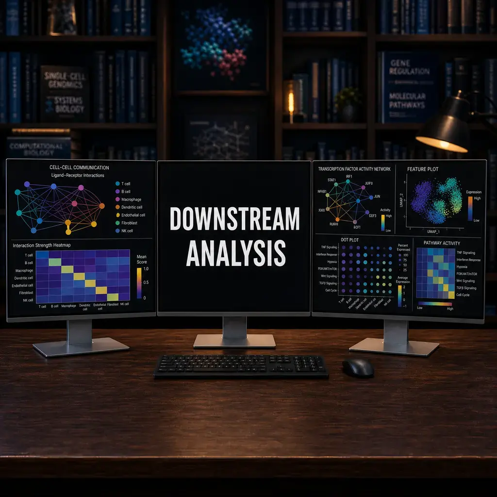
Once cells are clustered and annotated, the focus shifts to understanding how these populations function and interact. This involves interrogating Transcription Factor (TF) activity, inferring Cell-Cell Communication, and creating high-quality visualizations.

In this tutorial, we cover the foundational tools for these advanced downstream steps across both R and Python.

1. Cell-Cell Communication (Receptor-Ligand)

To understand how populations (e.g., T-cells and Macrophages) interact, we can map the expression of known Ligand-Receptor pairs. CellChat (R) and CellPhoneDB (Python) are the industry standards.

library(CellChat)
library(patchwork)

# 1. Create CellChat object from Seurat
cellchat <- createCellChat(object = pbmc, group.by = "ident")

# 2. Set the ligand-receptor database
CellChatDB <- CellChatDB.human
cellchat@DB <- CellChatDB

# 3. Preprocessing and Network Inference
cellchat <- subsetData(cellchat)
cellchat <- identifyOverExpressedGenes(cellchat)
cellchat <- identifyOverExpressedInteractions(cellchat)
cellchat <- computeCommunProb(cellchat)

# Filter out interactions in very few cells
cellchat <- filterCommunication(cellchat, min.cells = 10)

# Calculate aggregated communication network
cellchat <- computeCommunProbPathway(cellchat)
cellchat <- aggregateNet(cellchat)

# 4. Visualization (Circle Plot)
groupSize <- as.numeric(table(cellchat@idents))
netVisual_circle(cellchat@net$count, vertex.weight = groupSize,
                 weight.scale = T, label.edge= F, title.name = "Number of interactions")

# In Python, CellPhoneDB is typically run via the command line on exported count matrices.
# First, export your Scanpy AnnData object to raw counts and metadata.

import pandas as pd
import scanpy as sc

# Export metadata
df_meta = pd.DataFrame(adata.obs['leiden'])
df_meta['cell'] = df_meta.index
df_meta = df_meta[['cell', 'leiden']]
df_meta.to_csv('meta.tsv', sep='\t', index=False)

# Export counts
counts = pd.DataFrame(adata.raw.X.toarray(), index=adata.obs.index, columns=adata.raw.var_names)
counts = counts.T
counts.to_csv('counts.tsv', sep='\t')

# Run CellPhoneDB via terminal
cellphonedb method statistical_analysis meta.tsv counts.tsv \
    --counts-data=hgnc_symbol \
    --output-path=out_cpdb \
    --threads=8

2. Transcription Factor (TF) Activity

Gene expression alone doesn't prove a Transcription Factor is active. Using tools like Decoupler (Python) or DoRothEA (R), we can infer TF activity based on the expression of its known downstream target genes.

import decoupler as dc
import scanpy as sc

# 1. Retrieve the DoRothEA gene regulatory network (GRN) for humans
net = dc.get_dorothea(organism='human', levels=['A','B','C'])

# 2. Run multivariate linear model (MLM) to estimate TF activities
# We use the raw, log-normalized counts
dc.run_mlm(mat=adata, net=net, source='source', target='target', weight='weight', verbose=True)

# The results are stored in obsm. We can visualize the activity of a specific TF (e.g., STAT1)
sc.pl.umap(adata, color='STAT1', cmap='RdBu_r', vcenter=0)

library(dorothea)
library(Seurat)

# 1. Load the human regulons (confidence levels A, B, C)
dorothea_regulon_human <- get(data("dorothea_hs", package = "dorothea"))
regulon <- dorothea_regulon_human %>%
    dplyr::filter(confidence %in% c("A", "B", "C"))

# 2. Run VIPER algorithm to calculate TF activity
pbmc <- run_viper(pbmc, regulon,
                  options = list(method = "scale", minsize = 4,
                                 eset.filter = FALSE, cores = 1, verbose = FALSE))

# 3. Visualize TF activity
DefaultAssay(pbmc) <- "dorothea"
FeaturePlot(pbmc, features = "STAT1", cols = c("blue", "white", "red"))

3. Publication-Ready Plotting (SCpubr)

While Seurat's base plotting functions are good, the SCpubr package in R generates highly polished, publication-ready graphics automatically.

library(SCpubr)

# Generate a premium UMAP with custom labels, density contours, and refined aesthetics
SCpubr::do_DimPlot(sample = pbmc,
                   group.by = "ident",
                   label = TRUE,
                   label.box = TRUE,
                   repel = TRUE,
                   font.size = 14,
                   legend.position = "none")

# Generate a publication-quality DotPlot for marker genes
markers <- c("CD3D", "IL7R", "CD8A", "MS4A1", "CD14")
SCpubr::do_DotPlot(sample = pbmc,
                   features = markers,
                   group.by = "ident",
                   colors.use = c("lightgrey", "darkblue"))

Conclusion

Mastering these downstream analysis techniques allows you to graduate from simply classifying cells to understanding the mechanistic networks and interactions driving tissue biology. Both R and Python offer robust, highly developed tools to accomplish these goals.