Multi-Omics: CITE-seq & WNN Integration

Multi-Omics: CITE-seq & WNN Integration

Introduction

Traditional scRNA-seq only measures the transcriptome. However, many critical biological processes are driven by cell surface proteins (e.g., CD4, CD8, PD-1) whose abundance does not always correlate perfectly with RNA levels.

CITE-seq (Cellular Indexing of Transcriptomes and Epitopes by Sequencing) solves this by using antibody-derived tags (ADTs) to simultaneously measure RNA and protein levels in the exact same cell.

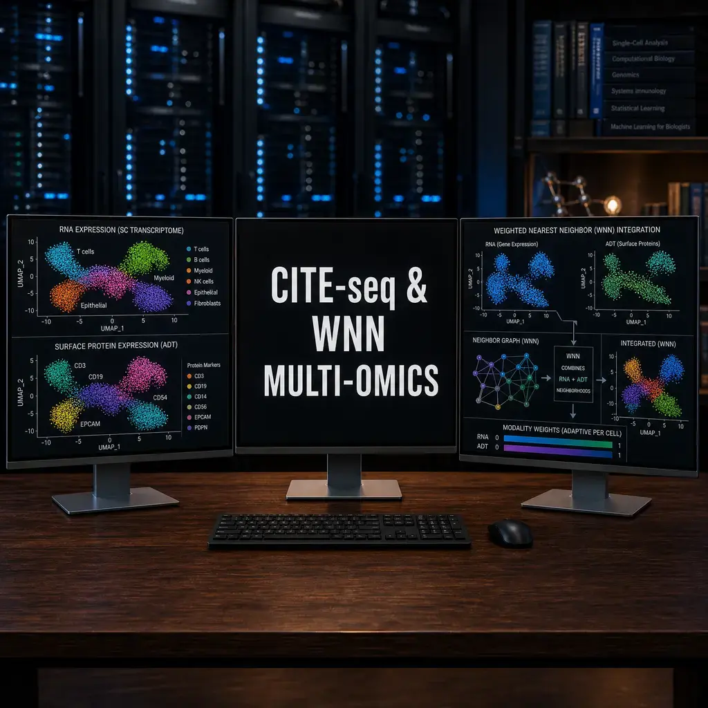
This tutorial covers the normalization of ADT data and the advanced Weighted Nearest Neighbor (WNN) integration method in Seurat to combine these two modalities.

1. Preparing the CITE-seq Object

A CITE-seq Seurat object contains two distinct "Assays": RNA (for transcripts) and ADT (for proteins).

library(Seurat)
library(ggplot2)

# Assuming 'seurat_obj' has already been loaded with both matrices
# Verify the assays
Assays(seurat_obj)
# Output should show: "RNA", "ADT"

2. ADT Normalization (Margin 1 vs Margin 2)

While RNA is usually normalized via LogNormalize or SCTransform, ADT data requires Centered Log-Ratio (CLR) normalization.

There are two ways to apply CLR: * Margin = 1 (Across cells): Normalizes the protein signal across all cells independently. Best when you want to compare the expression of a specific protein across different cell populations. * Margin = 2 (Across proteins): Normalizes the signal across all proteins within a single cell. Best for reducing cell-to-cell technical variations.

# Set Default Assay to ADT
DefaultAssay(seurat_obj) <- 'ADT'

# Normalize using CLR (Margin 2 is standard for CITE-seq in Seurat v4+)
seurat_obj <- NormalizeData(seurat_obj, normalization.method = 'CLR', margin = 2)

# Run PCA specifically on the protein data
# (Unlike RNA, we do not find variable features; we use all ADT proteins)
seurat_obj <- ScaleData(seurat_obj)
seurat_obj <- RunPCA(seurat_obj, features = rownames(seurat_obj), reduction.name = 'apca')

3. Weighted Nearest Neighbor (WNN) Integration

How do you combine RNA and Protein clustering? If you simply merge them, one modality will dominate the other.

Seurat's WNN Analysis solves this by calculating a "weight" for each cell. If a cell has a very clear protein profile but a noisy RNA profile, WNN assigns higher weight to the protein data for that specific cell.

# Ensure RNA has also been processed (SCTransform or LogNormalize + PCA)
DefaultAssay(seurat_obj) <- 'RNA'

# Find the multi-modal neighbors using WNN
seurat_obj <- FindMultiModalNeighbors(
  seurat_obj,
  reduction.list = list("pca", "apca"), # RNA PCA and ADT PCA
  dims.list = list(1:30, 1:18),         # Dimensions to use for each
  modality.weight.name = "RNA.weight"   # Name of the weight column
)

# Run UMAP and Clustering on the integrated WNN graph
seurat_obj <- RunUMAP(seurat_obj, nn.name = "weighted.nn", reduction.name = "wnn.umap", reduction.key = "wnnUMAP_")
seurat_obj <- FindClusters(seurat_obj, graph.name = "wsnn", algorithm = 3, resolution = 0.5)

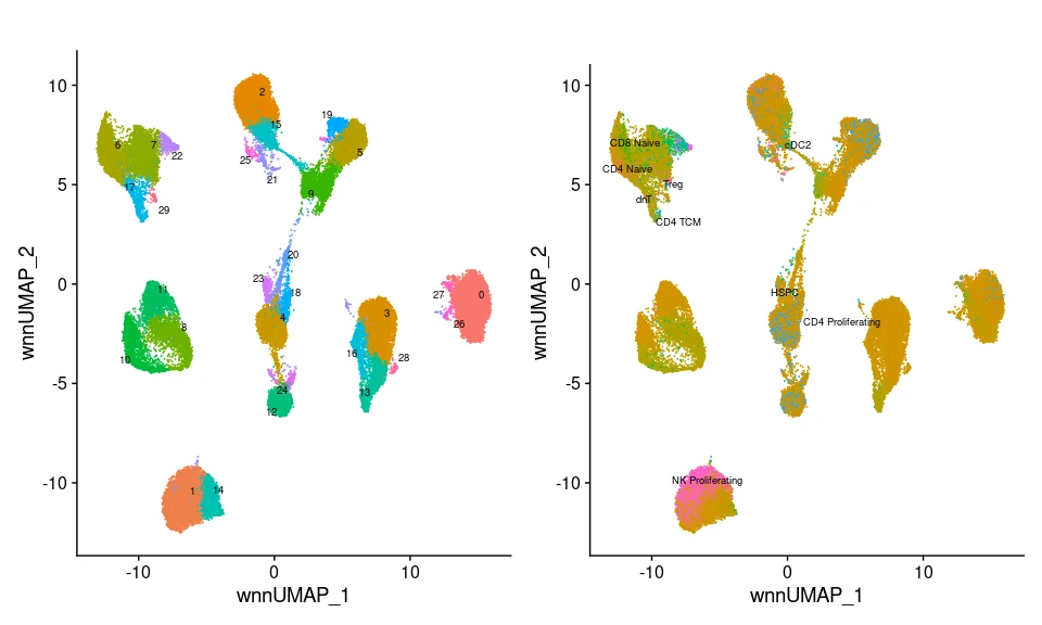
4. Visualizing Multi-Omics Data

Once WNN is complete, you can visualize both modalities side-by-side to see how surface proteins perfectly define clusters that RNA alone struggles to separate (such as CD4+ Memory vs Naive T-cells).

# Visualize the WNN UMAP
DimPlot(seurat_obj, reduction = 'wnn.umap', group.by = 'seurat_clusters', label = TRUE)

# Compare RNA vs Protein expression directly
FeaturePlot(seurat_obj,
            features = c("rna_CD4", "adt_CD4"), # Prefix determines the assay
            reduction = 'wnn.umap',
            min.cutoff = 'q10',
            max.cutoff = 'q90')

By leveraging WNN integration, you unlock a much higher resolution of cellular heterogeneity than standard scRNA-seq can provide.

Matched Python and R weighted-nearest-neighbour workflow

Preprocess RNA and protein modalities separately before computing a joint graph. Compare modality weights and marker evidence before interpreting the resulting clusters.

import muon as mu
import scanpy as sc

sc.pp.neighbors(mdata["rna"])
sc.pp.neighbors(mdata["prot"])
mu.pp.neighbors(mdata, key_added="wnn")
mu.tl.umap(mdata, neighbors_key="wnn")
sc.tl.leiden(mdata, neighbors_key="wnn", key_added="leiden_wnn")

library(Seurat)

seurat_obj <- FindMultiModalNeighbors(
  seurat_obj,
  reduction.list = list("pca", "apca"),
  dims.list = list(1:30, 1:18),
  modality.weight.name = "RNA.weight"
)
seurat_obj <- RunUMAP(seurat_obj, nn.name = "weighted.nn", reduction.name = "wnn.umap")
seurat_obj <- FindClusters(seurat_obj, graph.name = "wsnn", resolution = 0.5)