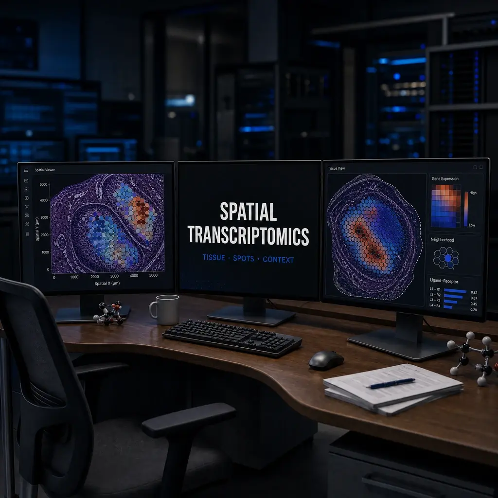
Spatial Transcriptomics

Tested on: Python 3.11, R 4.3.2, Ubuntu 24.04

Last Review: 2026-08-15

Learning Objectives & Prerequisites

Prerequisites: Complete scRNA-seq Basics and understand tissue sections, spatial coordinates, counts, and histology-aware interpretation.
Objective: Load, QC, visualize, and interpret spatial transcriptomics data while separating spatial association from causal tissue mechanisms.
Expected Output: A spatial plot with tissue context, QC notes, coordinate system, feature choice, and a cautious biological interpretation.

Suggested route: use the Bioinformatics Learning Path to review any prerequisite stage before continuing.

Spatial Transcriptomics: Bridging RNA and Anatomy

Introduction to Spatial Biology

Traditional single-cell RNA-seq requires dissociating tissues, which destroys the physical architecture and context of the cells. Spatial Transcriptomics (such as 10x Genomics Visium or Xenium) solves this by mapping gene expression directly onto intact histological tissue slices (like H&E stains).

This tutorial provides the foundational workflows for processing spatial data in both R and Python.

1. Loading and Preprocessing Spatial Data

Spatial data objects are unique because they contain two distinct types of data: the gene expression matrix (counts) and the spatial coordinates/images.

Both ecosystems load the same count matrix and spatial metadata, but store them in different object types.

import scanpy as sc
import squidpy as sq

adata = sq.read.visium("visium_brain_data/")
sc.pp.normalize_total(adata, inplace=True)
sc.pp.log1p(adata)
sc.pp.highly_variable_genes(adata, flavor="seurat", n_top_genes=2000)

library(Seurat)
library(ggplot2)

spatial_data <- Load10X_Spatial(data.dir = "visium_brain_data/")
spatial_data <- SCTransform(spatial_data, assay = "Spatial", verbose = FALSE)

2. Visualizing Gene Expression on Tissue

The power of spatial transcriptomics is seeing exactly where a gene is highly expressed across the physical tissue.

Use a feature plot to overlay a marker signal on the tissue image; report the gene symbol convention, image alignment, and color scale.

sc.pl.spatial(adata, color=["Snap25", "Mbp"], alpha_img=0.5, cmap="magma")

SpatialFeaturePlot(spatial_data, features = c("Snap25", "Mbp")) +
  theme(legend.position = "right")

3. Spatial Clustering

Just like scRNA-seq, we can cluster the "spots" based on their transcriptional profiles to find spatial domains (e.g., cortical layers in a brain, or tumor microenvironments).

Spatial clustering should be compared with tissue morphology and QC patterns. In Python, construct the spatial graph explicitly before using spatial statistics.

sc.tl.pca(adata)
sc.pp.neighbors(adata)
sc.tl.leiden(adata, key_added="clusters")
sq.gr.spatial_neighbors(adata)
sc.pl.spatial(adata, color="clusters", alpha_img=0.4)

spatial_data <- RunPCA(spatial_data, assay = "SCT", verbose = FALSE)
spatial_data <- FindNeighbors(spatial_data, reduction = "pca", dims = 1:30)
spatial_data <- FindClusters(spatial_data, verbose = FALSE)
SpatialDimPlot(spatial_data, label = TRUE, label.size = 3)

Summary

Both ecosystems are incredibly powerful. Seurat (R) provides an easy, out-of-the-box experience that is very familiar if you already do scRNA-seq. Squidpy (Python) provides superior tools for graph-based spatial statistics, such as testing if two cell types physically co-occur in the tissue.

Why Spatial Context Changes Everything

Standard single-cell RNA sequencing dissolves tissue into a suspension of individual cells. You recover transcriptomic profiles for thousands of cells, but you lose the one thing that is often biologically decisive: where each cell sat in the original tissue. Spatial transcriptomics restores that coordinate information. Each spot or bead in a Visium slide, or each pixel in a MERFISH experiment, carries both a gene expression vector and a physical position on the tissue section.

This matters enormously in cancer biology, neuroscience, and developmental biology. A macrophage sitting at the invasive front of a tumor behaves differently from a macrophage in the necrotic core, even if their bulk transcriptomes look similar. A neuron in layer II of the cortex expresses a different set of markers than a morphologically identical neuron in layer VI. Spatial methods let you ask which genes are enriched at tissue boundaries, which cell types co-localise with others, and whether a ligand-receptor interaction inferred from scRNA-seq data actually occurs between cells that are physically adjacent.

Choosing the Right Platform

The two most common approaches in 2026 are capture-based methods like 10x Genomics Visium and imaging-based methods like MERFISH, seqFISH, and Xenium. Visium captures all polyadenylated RNA across the transcriptome, but each spot averages roughly 5 to 15 cells. MERFISH and Xenium measure a curated panel of a few hundred to a few thousand genes at single-cell or subcellular resolution. The choice depends on your question: if you want transcriptome-wide discovery, use Visium; if you want to resolve individual cells with a targeted panel, use an imaging platform.

For Visium data, the standard analysis stack uses Seurat in R or Squidpy and Scanpy in Python. Both load the tissue image alongside the spot-by-gene count matrix, allowing you to overlay expression patterns directly onto the histological image. The key difference from scRNA-seq is that you must decide early whether to treat spots as pseudo-cells or to deconvolve them into constituent cell types using a reference single-cell atlas.

Deconvolution: Recovering Cell-Type Proportions from Spots

Because each Visium spot contains multiple cells, spatially variable genes are not necessarily cell-type-specific genes. A gene may appear enriched in a particular region simply because that region contains more of a given cell type, not because that gene is upregulated in those cells. Tools like RCTD, Spotlight, and NNLS deconvolution use a reference single-cell dataset to estimate the mixture of cell types in each spot. The result is a proportion matrix: for each spot, you obtain an estimate of how much of the signal comes from each cell type.

Once you have cell-type proportions, you can ask spatially resolved questions: do T cells and tumour cells co-localise? Do fibroblasts cluster near the stromal boundary? Which regions are predominantly composed of which cell types? These questions are not answerable from single-cell data alone, and they are what make spatial transcriptomics genuinely complementary rather than redundant with scRNA-seq.

Common Pitfalls and How to Avoid Them

One frequent mistake is treating spatially variable genes as differentially expressed genes without accounting for spatial autocorrelation. Standard differential expression tests assume independence between observations; adjacent spots share signal because they share cells at their edges. Tools like SpatialDE and NNSVG test for spatial variability directly, using statistical models that account for this autocorrelation.

Another pitfall is neglecting tissue quality. RNA degrades rapidly after tissue removal, and sections with high background fluorescence or poor morphology will produce noisy data regardless of the analysis method. Always inspect the histological image alongside QC metrics before committing to a dataset. A saturated or compressed tissue section will introduce artefacts that no computational method can fully correct.

When to Use Spatial Transcriptomics vs Standard scRNA-seq

Use spatial transcriptomics when tissue architecture is central to your hypothesis.
Use scRNA-seq when you need transcriptome-wide profiling at true single-cell resolution with high cell numbers.
Combine both when you want to annotate cell types from scRNA-seq and then map them back onto tissue using spatial data.

Knowledge Check & Assessment

1. Concept Verification

Why does spatial co-localization support a hypothesis but not prove direct cellular interaction or lineage?

2. Practical Execution

Load a small spatial dataset, plot a quality metric and one marker, then describe the tissue region and uncertainty in the observed pattern. Pass Criteria: Record the command or analysis choice, keep the output, and explain why it answers the stated task.

3. Troubleshooting

If a spatial pattern follows low capture or tissue-edge regions, how will you inspect spot QC, histology alignment, sequencing depth, and segmentation assumptions?